Quick Start
This “quick start” page is designed to introduce a few commonly-used features that you should know immediately as a user of WrightTools. At the beginning, we assume that you have installed WrightTools but are somewhat new to Python. If you are brand new to Python, it’s typically useful to run Python within an integrated development environment - our favorite is Spyder.
Each of the following code blocks builds on top of the previous code. Read this document like a series of commands typed into a Python shell. We recommend following along on your own machine.
We will introduce some important basics of WrightTools:
Create a Data Object
There are many ways to create a WrightTools data object. One strategy is to create a data object from your own data. Another is to open an existing wt5 file. First, we will explore importing your own data.
We provide an example infrared spectrum for you to manipulate here. Once you access this page, right click and save this file to your computer in an easily findable directory.
Now, open up your favorite Python IDE so you can continue. First, make sure that WrightTools is imported:
>>> import WrightTools as wt
>>> import pathlib
The next step is easier than you think. Identify the location of your file. For example, on Windows, if your username is user and the file is on your Desktop, then as far as Python is concerned, the file location is
r'C:\Users\user\Desktop\IR_spec.dpt'
Note that I renamed the file to “IR_spec.dpt” to make it easier to plug into my script. I find it easiest to do this in Notepad (open in Notepad, then save as “all files” and name the file IR_spec.dpt”). I added the ‘r’ in front of the path directory to let pathlib know this is a Windows directory.
We now need to import the file and (importantly) define it as a variable / data object. If the file is not imported as a data object, WrightTools will be confused. This is very important – if the file is not imported into WrightTools as a data object, nothing useful will happen.
To do this, we can use an import data command. Fortunately, the data object for a Bruker Tensor 27 Infrared Spectrometer is already programmed into WrightTools, which eases the import process.
For simplicity, I will define the data object as “d”. Then, to import this file into WrightTools, one simply types:
>>> d = wt.data.from_Tensor27(r'C:\Users\user\Desktop\IR_spec.dpt')
If you are successful, you will receive the following output:
range: 3999.21896 to 499.54073 (wn)
size: 7259
The final useful step here is to save as a .wt5 file, the natural file format of WrightTools. To do this, simply issue the command:
d.save('file_name')
where you substitute file_name with what you intend to name the dataset. This will save it in the original directory as a .wt5 file. To reopen the file, you simply issue the command:
d = wt.open('file_name.wt5')
Data manipulation can be done on this ‘d’ object, which is what we will explore below.
Creating a Quick and Dirty 1D Plot
In WrightTools, there are a variety of methods for plotting. Below, you can interact with some pre-installed data objects to explore these options. For now, we will stick to the IR Spectrum imported above.
To create a quick and dirty 1D plot, the command is
>>> wt.artists.quick1D()
In the parentheses, you insert your data object. Recall that we imported this infrared spectrum and identified it in WrightTools as a data object called “d”. Therefore, to make a quick 1D plot, simply issue the command
>>> wt.artists.quick1D(d)
And that is it! This is how you can easily graph 1D data in WrightTools from your own data sets. To see all the wonderful data formats supported by WrightTools, please access this page. In general, you can use wt.data.from_x, and replace x with the relevant instrument of interest. See the above page for more information.
Creating a Quick and Dirty 2D Plot
quick2D()
is built with the same goals as quick1D(),
but for two dimensional representations.
This time, we have to specify two axes to plot along—w1=wm and d2, in this example.
Again, we use the at keyword argument so only one plot will be generated.
We need to open a data object which involves a 2D data set. The FT-IR spectrum you manipulated above is NOT a 2D data set, but we provide a variety of published data sets for manipulation purposes.
We have stored these in a collection ‘datasets’. We open an arbitrary dataset as:
import matplotlib.pyplot as plt
import WrightTools as wt
from WrightTools import datasets
p = datasets.wt5.v1p0p1_MoS2_TrEE_movie
data = wt.open(p)
Let us see what channels we can plot with. This lets us choose, in the quick2D method, which axes we plot and furthermore, the data to be plotted as a function of these two axes. We do this by printing the tree of the data object, or
>>> data.print_tree()
Issuing this command yields the following information:
_001_dat ()
 ├── axes
 │   ├── 0: w2 (nm) (41, 1, 1)
 │   ├── 1: w1=wm (nm) (1, 41, 1)
 │   └── 2: d2 (fs) (1, 1, 23)
 ├── constants
 ├── variables
 │   ├── 0: w2 (nm) (41, 1, 1)
 │   ├── 1: w1 (nm) (1, 41, 1)
 │   ├── 2: wm (nm) (1, 41, 1)
 │   ├── 3: d2 (fs) (1, 1, 23)
 │   ├── 4: w3 = 800.0 (nm)
 │   ├── 5: d0 = 0.0 (fs)
 │   └── 6: d1 = -1.809751569485037 (fs)
 └── channels
     ├── 0: ai0 (41, 41, 23)
     ├── 1: ai1 (41, 41, 23)
     ├── 2: ai2 (41, 41, 23)
     ├── 3: ai3 (41, 41, 23)
     ├── 4: ai4 (41, 41, 23)
     └── 5: mc (41, 41, 23)
So, we have 3 possible axes (w1, w2, d2) and 5 channels (ai0, ai1, ai2, ai3, ai4, ai5). By default, WrightTools will plot the first channel (ai0) in a quick2D plot. So let’s give it a whirl by plotting this data. Let’s plot the data with one axis as w1, the second axis as d2, and choose the third channel (w2) to be constant at 2 eV. This last constraint is important because this is a 3D data set - for each w1, w2, or d2 value, we can produce a 2D plot. So we simply choose a single w2 value (2 eV) to understand the spectral response at that specific point (w1, d2, 2 eV) = (w1, d2, w2).
Now we have enough to create the 2D plot. By issuing the commands:
wt.artists.quick2D(data, 'w1=wm', 'd2', at={'w2': [2, 'eV']})
plt.show()
import matplotlib.pyplot as plt
import WrightTools as wt
from WrightTools import datasets
p = datasets.wt5.v1p0p1_MoS2_TrEE_movie
data = wt.open(p)
wt.artists.quick2D(data, 'w1=wm', 'd2', at={'w2': [2, 'eV']})
plt.show()
(Source code, png, pdf)
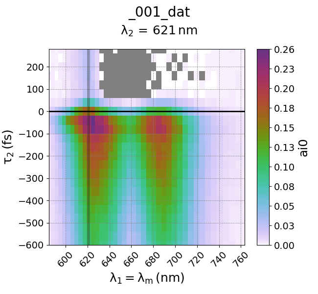
This should yield the plot as described above. Note that WrightTools is smart enough to automatically convert units! You can alternatively forcibly induce a unit change through
w2.unit_convert('eV')
Process Data
Now let’s actually modify the arrays that make up our data object. Note that the raw data which we imported is not being modified, rather we are modifying the data as copied into our data object.
Convert
As we saw above, WrightTools has built in units support. This enables us to easily convert our data object from one unit system to another:
>>> data.units
('nm', 'nm', 'fs')
>>> data.convert('eV')
axis w2 converted from nm to eV
axis w1=wm converted from nm to eV
>>> data.units
('eV', 'eV', 'fs')
Note that only compatable axes were converted—the trailing axis with units 'fs' was ignored.
Want fine control?
You can always convert individual axes, e.g. data.w2.convert('wn').
For more information see Units.
Split
Use split() to break your dataset into smaller pieces. This is useful if you want to look at specific regions.
Consider the above 3D data object that we just used to create a 2D plot. Let’s say we are only interested in d2 dynamics after d2 = 0. We split the d2 axis at d2 = 0, which will yield two new objects: before 0 and after 0.
To do this, we need to introduce a new data object, which we will call col. We thus split the data as follows:
>>> col = data.split('d2', 0.)
split data into 2 pieces along <d2>:
  0 : -inf to 0.00 fs (1, 1, 15)
  1 : 0.00 to inf fs (1, 1, 8)
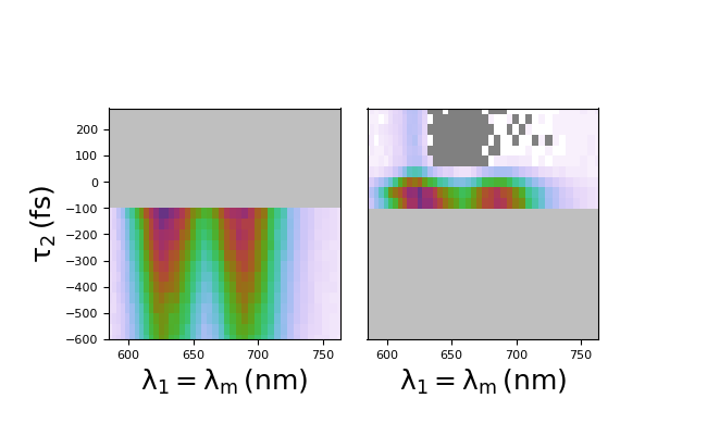
Now, col is an object which has two components, col.split000 and col.split001. These are d2<0 and d2>0, respectively. To plot the data of interest, d2 > 0, we simply employ the quick2D code before and plot col.split001.
You can additionally employ for loops and other methods to create a program which automatically splits the data and plots them individually, as seen below.
import matplotlib.pyplot as plt
import WrightTools as wt
from WrightTools import datasets
p = datasets.wt5.v1p0p1_MoS2_TrEE_movie
data = wt.open(p)
col = data.split('d2', -100.)
fig, gs = wt.artists.create_figure(cols=[1,1])
for i, d in enumerate(col.values()):
    d = d.chop("w1=wm", "d2", at={"w2": (2, "eV")})[0]
    ax = plt.subplot(gs[i])
    ax.pcolor(d)
    ax.set_xlim(data.w1__e__wm.min(), data.w1__e__wm.max())
    ax.set_ylim(data.d2.min(), data.d2.max())
wt.artists.set_fig_labels(xlabel=data.w1__e__wm.label, ylabel=data.d2.label)
plt.show()
Note that split() accepts axis expressions and unit-aware coordinates, not axis indices.
import matplotlib.pyplot as plt
import WrightTools as wt
from WrightTools import datasets
p = datasets.wt5.v1p0p1_MoS2_TrEE_movie
data = wt.open(p)
col = data.split('d2', -100.)
fig, gs = wt.artists.create_figure(cols=[1,1])
for i, d in enumerate(col.values()):
    d = d.chop("w1=wm", "d2", at={"w2": (2, "eV")})[0]
    ax = plt.subplot(gs[i])
    ax.pcolor(d)
    ax.set_xlim(data.w1__e__wm.min(), data.w1__e__wm.max())
    ax.set_ylim(data.d2.min(), data.d2.max())
wt.artists.set_fig_labels(xlabel=data.w1__e__wm.label, ylabel=data.d2.label)
plt.show()
(Source code, png, pdf)

Clip
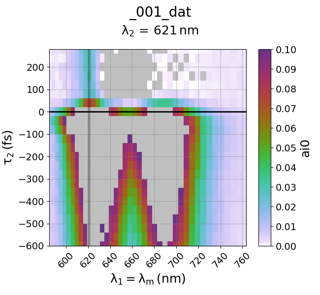
Use clip() to ignore/remove points of a channel outside of a specific range. For example, if you are interested in only looking at less intense values in a spectrum, you can cut out (clip) the larger values of interest. For example, if you would like to only look at spectral values with intensity between 0 to 0.1, we simply need to clip the intensity values larger than that.
We perform this through the command
data.ai0.clip(min=0.0, max=0.1)
This effectively constrains all plotted values between 0 to 0.1. We can plot it as follows:
import matplotlib.pyplot as plt
import WrightTools as wt
from WrightTools import datasets
p = datasets.wt5.v1p0p1_MoS2_TrEE_movie
data = wt.open(p)
data.ai0.clip(min=0.0, max=0.1)
wt.artists.quick2D(data, 'w1=wm', 'd2', at={'w2': [2, 'eV']})
plt.show()
import matplotlib.pyplot as plt
import WrightTools as wt
from WrightTools import datasets
p = datasets.wt5.v1p0p1_MoS2_TrEE_movie
data = wt.open(p)
data.ai0.clip(min=0.0, max=0.1)
wt.artists.quick2D(data, 'w1=wm', 'd2', at={'w2': [2, 'eV']})
plt.show()
(Source code, png, pdf)

Transform
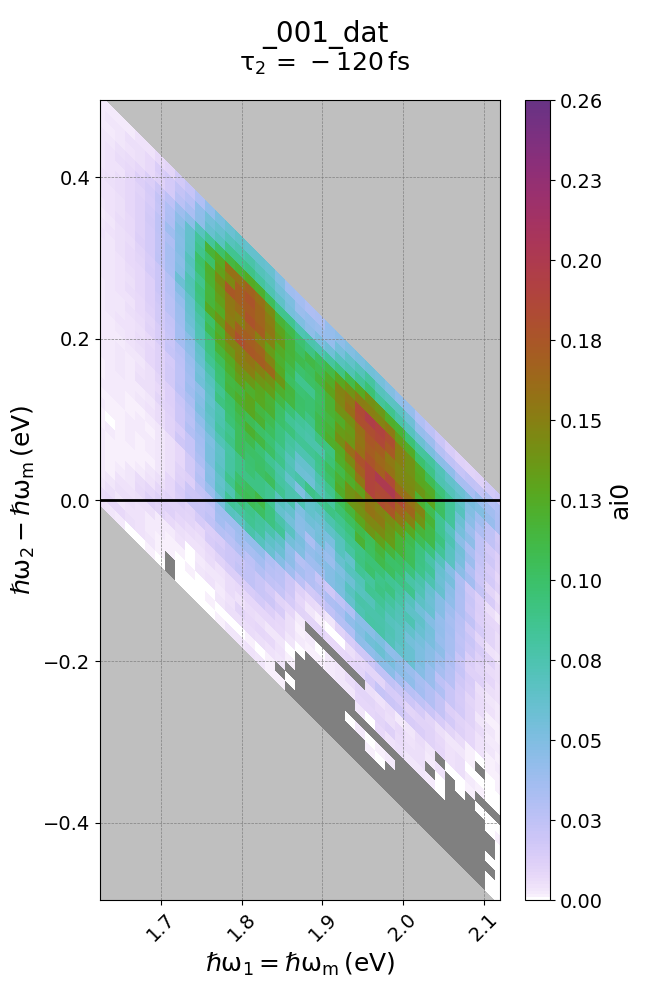
Use transform() to choose a different set of axes for your data object. For example, you have a data set of axes w1 and w2. Pretend for example you have a spectral object that should exist at w2 = w + w1. If we believe this, we can transform the axes to generate a plot that will explicitly show the ‘w’ frequency, instead of the w2 axis. This makes it easier to plot.
We perform this through the data transform. Importing the data object as ‘data’, we issue the command:
data.transform('w1=wm', 'w2-wm', 'd2')
Note that this did exactly as intended. Since w1 was transformed as being identical to wm, the transformation w2 -> w2 - wm is identical to w, as w = w2 - wm = w2 - w1. The resultant spectrum (plotted below) makes this clear.
import matplotlib.pyplot as plt
import WrightTools as wt
from WrightTools import datasets
p = datasets.wt5.v1p0p1_MoS2_TrEE_movie
data = wt.open(p)
data.transform('w1=wm', 'w2-wm', 'd2')
data.convert('eV')
wt.artists.quick2D(data, 'w1=wm', 'w2-wm', at={'d2': (-100, 'fs')})
plt.show()
(Source code, png, pdf)
Creating a 1D plot from 2D data objects
The idea is here is that you are interested in spectral information across a certain axis. For example, let’s say you should see many modes coupled to w1 = 1.5 eV. We can effectively create a 1D spectrum with w1 stagnant at 1.5 eV and w2 spanning its entire range to identify coupled features.
This method employs all the tricks from above. We first chop the data at specific w1 values:
data1 = data.chop('w2', at={'w1=wm':[1.5, 'eV']})[0]
Since we have multiple data1 values (at different delays – we have many d2 points!) we just choose an arbitrary one. For laziness, we choose the first point, so we add the [0] index to the end. We can then plot this:
wt.artists.quick1D(data1)
To choose a specific time point, you can of course just make the chopping more specific. For example, to chop at d2 = 0:
data1 = data.chop('w2', at={'w1=wm':[1.5, 'eV'], 'd2':[0, 'fs']})[0]
import matplotlib.pyplot as plt
import WrightTools as wt
from WrightTools import datasets
p = datasets.wt5.v1p0p1_MoS2_TrEE_movie
data = wt.open(p)
data.transform('w1=wm', 'w2-wm', 'd2')
data.convert('eV')
data1 = data.chop('w2', at={'w1=wm':[1.5, 'eV'], 'd2':[0, 'fs']})[0]
wt.artists.quick1D(data1)
plt.show()
Collections
Collections are containers that can hold multiple data objects. Collections can nest within each-other, much like folders in your computers file system. Collections can help you store all associated data within a single wt5 file, keeping everything internally organized. Creating collections is easy:
>>> collection = wt.Collection(name='test')
Filling collections with data objects is easy as well.
Again, let’s use the WrightTools.datasets package:
>>> from WrightTools import datasets
>>> p = datasets.COLORS.v0p2_d1_d2_diagonal
>>> wt.data.from_COLORS(p, parent=collection)
cols recognized as v0 (19)
data created at /tmp/w1ijzsmv.wt5::/d1_d2_diagonal_dat
  axes: ('d1', 'd2')
  shape: (21, 21)
>>> p = datasets.ocean_optics.tsunami
>>> wt.data.from_ocean_optics(p, parent=collection)
data created at /tmp/w1ijzsmv.wt5::/tsunami
  range: 339.95 to 1013.55 (nm)
  size: 2048
>>> p = datasets.PyCMDS.wm_w2_w1_000
>>> wt.data.from_PyCMDS(p, parent=collection)
data created at /tmp/w1ijzsmv.wt5::/3d1580hi
  axes: ('wm', 'w2', 'w1')
  shape: (35, 11, 11)
Note that we are using from functions instead of open().
That’s because these aren’t wt5 files—they’re raw data files output by various instruments.
We use the parent keyword argument to create these data objects directly inside of our collection.
See Data for a complete list of supported file formats.
Much like data objects, collection objects have a method print_tree() that prints out a bunch of information:
>>> collection.print_tree()
test (/tmp/w1ijzsmv.wt5)
├── 0: d1_d2_diagonal_dat (21, 21)
│   ├── axes: d1 (fs), d2 (fs)
│   ├── constants:
│   └── channels: ai0, ai1, ai2, ai3
├── 1: tsunami (2048,)
│   ├── axes: energy (nm)
│   ├── constants:
│   └── channels: signal
└── 2: 3d1580hi (35, 11, 11)
    ├── axes: wm (wn), w2 (wn), w1 (wn)
    ├── constants:
    └── channels: signal_diff, signal_mean, pyro1, pyro2, pyro3, PMT voltage
Collections can be saved inside of wt5 files, so be aware that open() may return a collection or a data object based on the contents of your wt5 file.
Learning More
We hope that this quick start page has been a useful introduction to you. Now it’s time to go forth and process data! If you want to read further, consider the following links: